![[logo]](/images/SimplyGenius.png)
Simply Genius .NET
Software that makes you smile
Myers' Diff Algorithm : The basic greedy algorithm

|
|
Publicly recommend on Google
|
Table of Contents
Introduction
This article is an examination of the basic greedy diff algorithm, as described by Eugene W. Myers in his paper, "An O(ND) Difference Algorithm and Its Variations". It was published in the journal "Algorithmica" in November 1986. The paper is available as a PDF here[^].
In his paper, Myers also extends his basic algorithm with the "Linear Space Refinement". This requires a sound understanding of the basic algorithm as described in this article. It is examined in part II, which is available here [^].
The application available in the downloads is a learning aid. It displays a graphical representation of the various stages of the algorithm. I suggest you use it while reading this article to help understand the algorithm. The graphs in this article are screenshots of the application.
This article uses a character-by-character diff, but the algorithm can be used for any data type that has an equality operator.
Background
I started looking at diff algorithms for a competition held on The Code Project in August 2009. The more I learnt about Myers' algorithms, the more beautiful I found them. I thoroughly recommend spending some time investigating them. I have certainly enjoyed learning and implementing them.
I have written this article because it took me about a week to understand and implement the algorithm from the paper. You can read this article in less than an hour and I hope this will leave you with a general appreciation for Myers' work. I have tried to explain the necessary tenets and theory without giving proofs. These are available in Myers' paper.
Definitions
File A and File B
The diff algorithm takes two files as input. The first, usually older, one is file A, and the second one is file B. The algorithm generates instructions to turn file A into file B.
Shortest Edit Script ( SES )
The algorithm finds the Shortest Edit Script that converts file A into file B. The SES contains only two types of commands: deletions from file A and insertions in file B.
Longest Common Subsequence ( LCS )
Finding the SES is equivalent to finding the Longest Common Subsequence of the two files. The LCS is the longest list of characters that can be generated from both files by removing some characters. The LCS is distinct from the Longest Common Substring, which has to be contiguous.
For any two files, there can be multiple LCSs. For example, given the sequences "ABC" and "ACB", there are two LCSs of length 2: "AB" and "AC". An LCS corresponds directly to an SES, so it is also true that there can be multiple SESs of the same length for any two files. The algorithm just returns the first LCS / SES that it finds, which therefore may not be unique.
Example sequences
This article uses the same example as the paper. File A contains "ABCABBA" and file B contains "CBABAC". These are represented as two character arrays: A[] and B[].
The length of A[] is N and the length of B[] is M.
Edit graph
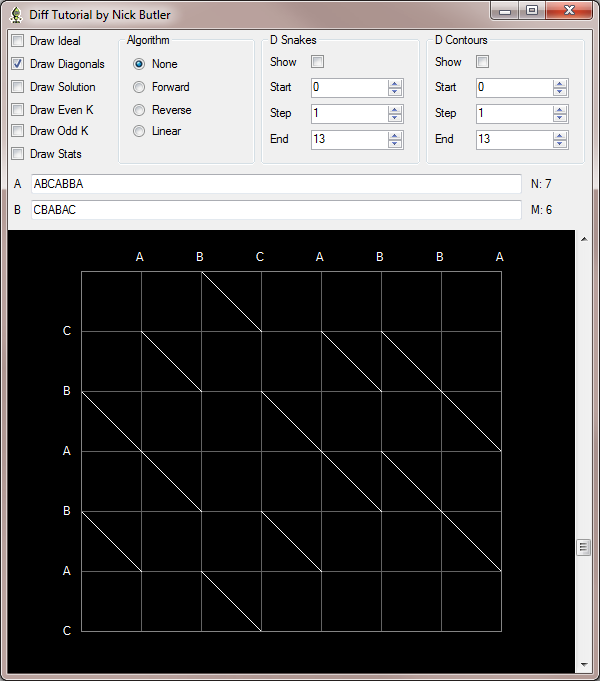
This is the edit graph for the example. Array A is put along the x-axis at the top. Array B is put along the y-axis reading downwards.
|
|
|
Figure 1 : Example edit graph
|
The solution is the shortest path from the top-left corner ( 0, 0 ) to the bottom-right corner ( 7, 6 ).
You can always move one character horizontally or vertically. A horizontal ( right ) move represents a deletion from file A, and a vertical ( down ) move represents an insertion in file B. If there is a matched character, then you can also move diagonally, ending at the match.
The solution(s) are the trace(s) that include the most diagonals. The LCS is the diagonals in the trace, and the SES is the horizontal and vertical moves in it. For the example, the LCS is 4 characters long and the SES is 5 differences long.
Snakes
The paper is slightly ambiguous, but I understand a snake to be defined as a single deletion or insertion followed by zero or more diagonals.
For the example, there are two snakes starting at the top-left ( 0, 0 ). One goes right to ( 1, 0 ) and stops. The other goes down to ( 0, 1 ) and stops. The next snake down from ( 0, 1 ) goes to ( 0, 2 ) and then along the diagonal to ( 2, 4 ). I call these points the start, mid, and end points, respectively.
k lines
You can draw lines starting at points on the x-axis and y-axis and parallel to the diagonals. These are called k lines and will be very useful. The line starting at ( 0, 0 ) is defined to be k = 0. k increases in lines to the right and decreases downwards. So the k line through ( 1, 0 ) has k = 1, and the k line through ( 0, 1 ) has k = -1.
In fact, they are the lines represented by the equation: y = x - k. This is also useful, because we only need to store the x value for a particular point on a given k line and we can simply calculate the y value.
d contours
A difference is shown by a horizontal or vertical move in the edit graph. A contiguous series of snakes has a d value which is the number of differences in that trace, irrespective of the number of diagonals in it. A d contour can be created that joins the end points of all traces with a given d value.
Greedy Algorithm
We will now examine the basic greedy algorithm, that is, without the linear space refinement.
|
|
|
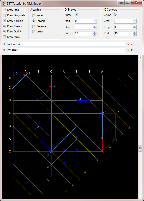
Figure 2: Forward greedy solution
|
Edit graph
This graph looks daunting but I will walk though it layer by layer.
- k lines: The brown lines are the k lines for odd values of k. The yellow lines are the k lines for even values of k.
- snakes: The dark blue lines are snakes. The red snakes show the solution trace.
- d contours: The light blue lines are difference contours. For example, the three end points on the line marked '2' all have exactly 2 horizontal or vertical moves.
Algorithm
The algorithm is iterative. It calculates the furthest reaching paths on each k line for successive d. A solution is found when a path reaches the bottom right corner. This is guaranteed to be an LCS / SES because we have already calculated all possibilities with smaller d. The maximum value of d is when there are no matches, which is N deletions + M insertions.
for ( int d = 0 ; d <= N + M ; d++ )
Inside this loop, we must find the furthest reaching path for each k line. For a given d, the only k lines that can be reached lie in the range [ -d .. +d ]. k = -d is possible when all moves are down, and k = +d is when all moves are to the right. An important observation for the implementation is that end points for even d are on even k lines and vice-versa. So, the inner loop is:
for ( int k = -d ; k <= d ; k += 2 )
So, the missing piece is how to find the furthest reaching path on a given k line.
The first thing to note is that to get on a line k, you must either move down from line k + 1 or right from line k - 1. If we save the furthest reaching paths from the previous d, we can choose the move that gets us furthest along our line k. The two edge cases are when k = -d, in which case you can only move down, and k = +d, when you can only move right.
Example when d = 3
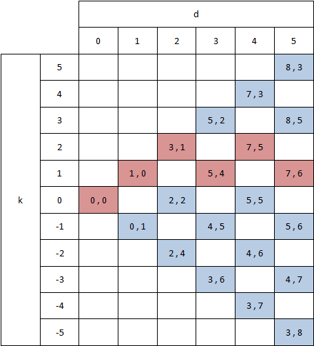
I will work through the example for d = 3 which means k lines [ -3, -1, 1, 3 ]. To help, I have transcribed the end points of the snakes in the example into the table below:
|
|
|
Figure 3: End point table
|
k = -3: It is impossible to get to line k = -4 when d = 2, so we must move down from line k = -2. Our saved result from the previous d = 2 gives our start point as ( 2, 4 ). The down move gives a mid point as ( 2, 5 ) and we have a diagonal which takes us to ( 3, 6 ).
k = -1: We have two options here. We can move right from k = -2 or down from k = 0. Looking at the results for the previous d = 2, the previous point on k = -2 is ( 2, 4 ) and the previous point on k = 0 is ( 2, 2 ). Moving right from k = -2 takes us to ( 3, 4 ) and moving down from k = 0 takes us to ( 2, 3 ). So we choose k = -2 as it gets us further along our line k = -1. We have a diagonal again, so our snake is ( 2, 4 ) -> ( 3, 4 ) -> ( 4, 5 ).
k = 1: We have two options again. We can move right from k = 0 or down from k = 2. The previous end points are ( 2, 2 ) and ( 3, 1 ), which both take us to ( 3, 2 ). We will arbitrarily choose to start from the point with the greater x value, which with the diagonal gives us the snake ( 3, 1 ) -> ( 3, 2 ) -> ( 5, 4 ).
k = 3: This is the other edge case. Line k = 4 is impossible with d = 2, so we have to move right from k = 2. Our previous result on k = 2 is ( 3, 1 ), so a right move takes us to ( 4, 1 ). We have a diagonal again, giving an end point at ( 5, 2 ).
Implementation
How can we implement this? We have our two loops, what we need is a data structure.
Notice that the solutions for d(n) only depend on the solutions for d(n - 1). Also remember that for even values of d, we find end points on even k lines, and these only depend on the previous end points which are all on odd k lines. Similarly for odd values of d.
So, we use an array called V with k as the index and the x position of the end point as the value. We don't need to store the y position, as we can calculate it given x and k: y = x - k. Also, for a given d, k is in the range [ -d .. d ], which are the indices into V and so limit its size.
This works well, because when d is even, we calculate the end points for even k indices using the odd k values which are immutable for this iteration of d. Similarly for odd values of d.
The decision whether to go down or right to get to a given k line can therefore be written as a boolean expression:
bool down = ( k == -d || ( k != d && V[ k - 1 ] < V[ k + 1 ] ) );
If k = -d, we must move down, and if k = d, we must move right. For the normal middle cases, we choose to start from whichever of the neighboring lines has the greater x value. This guarantees we reach the furthest possible point on our k line.
We also need a stub for d = 0, so we set V[ 1 ] = 0. This represents a point on line k = 1 where x = 0. This is therefore the point ( 0, -1 ). We are guaranteed to move down from this point, which takes us to ( 0, 0 ) as required.
So, here is the core implementation:
V[ 1 ] = 0;

for ( int d = 0 ; d <= N + M ; d++ )
{
  for ( int k = -d ; k <= d ; k += 2 )
  {
    // down or right?
    bool down = ( k == -d || ( k != d && V[ k - 1 ] < V[ k + 1 ] ) );

    int kPrev = down ? k + 1 : k - 1;

    // start point
    int xStart = V[ kPrev ];
    int yStart = xStart - kPrev;

    // mid point
    int xMid = down ? xStart : xStart + 1;
    int yMid = xMid - k;

    // end point
    int xEnd = xMid;
    int yEnd = yMid;

    // follow diagonal
    int snake = 0;
    while ( xEnd < N && yEnd < M && A[ xEnd ] == B[ yEnd ] ) { xEnd++; yEnd++; snake++; }

    // save end point
    V[ k ] = xEnd;

    // check for solution
    if ( xEnd >= N && yEnd >= M ) /* solution has been found */
  }
}
Solution
The code above finds the first snake that reaches the end of both sequences. However, the data in V only stores the latest end point for each k line. To find all the snakes that lead to the solution requires taking a snapshot of V after each iteration of d and then working backwards from dsolution to 0.
IList<V> Vs; // saved V's indexed on d
IList<Snake> snakes; // list to hold solution

POINT p = new POINT( N, M ); // start at the end

for ( int d = vs.Count - 1 ; p.X > 0 || p.Y > 0 ; d-- )
{
  var V = Vs[ d ];

  int k = p.X - p.Y;

  // end point is in V
  int xEnd = V[ k ];
  int yEnd = x - k;

  // down or right?
  bool down = ( k == -d || ( k != d && V[ k - 1 ] < V[ k + 1 ] ) );

  int kPrev = down ? k + 1 : k - 1;

  // start point
  int xStart = V[ kPrev ];
  int yStart = xStart - kPrev;

  // mid point
  int xMid = down ? xStart : xStart + 1;
  int yMid = xMid - k;

  snakes.Insert( 0, new Snake( /* start, mid and end points */ ) );

  p.X = xStart;
  p.Y = yStart;
}
It should be noted that this 'greedy' algorithm has complexity O( (N+M) D ) in both time and space.
Conclusion
I hope you have enjoyed reading this article as much as I have enjoyed writing it.
The second part of this article, which explores the linear space refinement, is available here [^].
History
- Sept. 2009: First edition.
License
This article, along with any associated source code and files, is licensed under The Code Project Open License.
Contact
If you have any feedback, please feel free to contact me.


